Regresión lineal simple

Diseño experimental

Bibliotecas

library(tidyverse)
library(ggpubr)
library(qqplotr)

Datos

• Fuente de datos

datos <- read_csv("datos/lecheria_eeuu.csv")
datos |> head()

• ¿Cuál es nuestra variable respuesta?
• ¿Cuál o cuáles variables son predictoras?

¿Normalidad?

ggqqplot(datos$avg_price_milk)

• Normalidad de todas las variables

datos |> 
  select(-year) |> 
  pivot_longer(cols = everything()) |> 
  ggplot(aes(sample = value)) +
  facet_wrap(~name, scales = "free") +
  stat_qq_band() +
  stat_qq_line() +
  stat_qq_point()

Correlación

Paramétrica (Pearson)

\[\rho_{(X,Y)} = \frac{Cov_{(X,Y)}}{\sigma_X\times\sigma_Y} = \frac{\sum_{i=1}^{n}(X_i-\mu_X)(Y_i-\mu_Y)}{\sigma_X\times\sigma_Y}\]

• Cálculo manual:

covarianza <- cov(x = datos$dairy_ration, y = datos$avg_price_milk)
desv_x <- sd(datos$dairy_ration)
desv_y <- sd(datos$avg_price_milk)

covarianza / (desv_x * desv_y)

[1] 0.8172358

• Cálculo con la función cor:

cor(x = datos$dairy_ration,
    y = datos$avg_price_milk)

[1] 0.8172358

No paramétrica (Spearman)

\[\rho = 1 - \frac{6\sum D^2}{N (N^2 - 1)}\]

• \(D\): diferencia entre los estadísticos de orden \(x - y\)

cor(x = datos$dairy_ration,
    y = datos$avg_price_milk,
    method = "spearman")

[1] 0.63335

Diagrama de dispersión

datos |> 
  ggplot(aes(x = dairy_ration, y = avg_price_milk)) +
  geom_point()

• Agregamos una línea de tendencia lineal:

datos |> 
  ggplot(aes(x = dairy_ration, y = avg_price_milk)) +
  geom_point() +
  geom_smooth(method = "lm")

• ¿Existe alguna relación no lineal?

datos |> 
  ggplot(aes(x = dairy_ration, y = avg_price_milk)) +
  geom_point() +
  geom_smooth()

Regresión lineal simple

• El propósito principal del análisis de regresión es estimar la función de regresión poblacional con base en la función de regresión muestral.

\[Y_i = \beta_0\ +\ \beta_1X\] \[\hat{Y_i} = \hat{\beta_0}\ + \hat{\beta_1}X_i\ + \hat{\epsilon_i}\]

• Función matemática:

\[Y_i = E(Y|X_i)\ +\ \epsilon_i\\\]

• Asumiendo que \(E(Y|X_i)\) es lineal en \(X_i\):

\[Y_i = E(Y|X_i)\ +\ \epsilon_i\\ Y_i = \beta_0 +\ \beta_1X_i\ +\ \epsilon_i\]

modelo1 <- lm(avg_price_milk ~ dairy_ration, data = datos)
modelo1 |> summary()

Call:
lm(formula = avg_price_milk ~ dairy_ration, data = datos)

Residuals:
      Min        1Q    Median        3Q       Max 
-0.033635 -0.008394 -0.002785  0.003106  0.055094 

Coefficients:
             Estimate Std. Error t value Pr(>|t|)    
(Intercept)  0.086176   0.007885  10.930 1.67e-12 ***
dairy_ration 1.038172   0.127443   8.146 2.10e-09 ***
---
Signif. codes:  0 '***' 0.001 '**' 0.01 '*' 0.05 '.' 0.1 ' ' 1

Residual standard error: 0.01655 on 33 degrees of freedom
Multiple R-squared:  0.6679,    Adjusted R-squared:  0.6578 
F-statistic: 66.36 on 1 and 33 DF,  p-value: 2.102e-09

Ecuación final

\[\hat{y} = 0.086176 + (1.038172 \times X)\]

• ¿Cuánto es el precio promedio esperado de la leche para una ración de 0.082?

0.086176 + (1.038172 * 0.082)

[1] 0.1713061

Predicción con R

datos_test <-
  datos |> 
  sample_n(size = 10) |> 
  select(dairy_ration)

datos_test

• Usamos la función predict con el modelo1 previamente ajustado:

predict(object = modelo1, 
        newdata = datos_test)

        1         2         3         4         5         6         7         8 
0.2077383 0.1315572 0.1384699 0.1373187 0.1978416 0.2123142 0.1384508 0.1360335 
        9        10 
0.1849064 0.1445377 

¿Cómo evalúo mi modelo?

Bondad de ajuste

• Coeficiente de determinación (R cuadrado - \(R^2\))

\[R^2 = \rho^2\]

correlacion_pearson <- 0.8172358
r2 <- correlacion_pearson ^ 2
r2

[1] 0.6678744

• Coeficiente de determinación ajustado:

\[R^2_a = 1 - \frac{N-1}{N-k-1} (1 - R^2)\]

N <- nrow(datos) # número de datos
k <- 1 # pendiente (parámetro Beta1)

1 - ((N - 1) / (N - k - 1)) * (1 - r2)

[1] 0.6578099

RMSE

• Raíz del error cuadrático medio

\[RMSE = \sqrt{\frac{\sum_{i = 1}^{n} (y - \hat{y})^2}{N}}\]

• Calculando manualmente el RMSE:

valores_reales <- datos$avg_price_milk # variable y
predichos_m1 <- modelo1$fitted.values

diferencia_cuadrado <- (valores_reales - predichos_m1)^2
suma_cuadrados <- sum(diferencia_cuadrado)
metrica_rmse <- sqrt(suma_cuadrados / N)
metrica_rmse

[1] 0.01606818

• Usando la biblioteca yardstick para calcular el RMSE:

library(yardstick)
rmse_vec(truth = valores_reales, estimate = predichos_m1)

[1] 0.01606818

AIC

• Criterio de información de Akaike

\[AIC = -2ln(L) + k\times n_{par}\]

• Cálculo manualmente:

log_l <- logLik(modelo1) # log verosimilitud
n_par <- length(coefficients(modelo1)) # número de parámetros

-2 * log_l + 2 * n_par

'log Lik.' -185.8383 (df=3)

• Cálculo con R:

AIC(modelo1)

[1] -183.8383

Análisis de residuales

• ¿Qué es exactamente un residual \((\epsilon_i)\)?

• Obtengamos los residuales desde nuestro modelo1:

residuales <- modelo1$residuals
residuales

            1             2             3             4             5 
-0.0063963730 -0.0004507765  0.0039146871 -0.0045249485 -0.0066020776 
            6             7             8             9            10 
-0.0058987810 -0.0003646907  0.0030543723 -0.0131944037 -0.0027847996 
           11            12            13            14            15 
 0.0004026023 -0.0107404425 -0.0005572382 -0.0059314158 -0.0073187107 
           16            17            18            19            20 
-0.0101901072 -0.0010347143 -0.0115376727  0.0197303289  0.0161825420 
           21            22            23            24            25 
-0.0051450271  0.0180051551 -0.0137001647 -0.0110334541  0.0208318798 
           26            27            28            29            30 
 0.0162116339 -0.0094699308  0.0342720367  0.0016622358 -0.0336354964 
           31            32            33            34            35 
 0.0020442379  0.0031583847 -0.0273141708 -0.0067382644  0.0550935636 

• ¿Cómo calculamos estos valores?

valores_reales - predichos_m1

            1             2             3             4             5 
-0.0063963730 -0.0004507765  0.0039146871 -0.0045249485 -0.0066020776 
            6             7             8             9            10 
-0.0058987810 -0.0003646907  0.0030543723 -0.0131944037 -0.0027847996 
           11            12            13            14            15 
 0.0004026023 -0.0107404425 -0.0005572382 -0.0059314158 -0.0073187107 
           16            17            18            19            20 
-0.0101901072 -0.0010347143 -0.0115376727  0.0197303289  0.0161825420 
           21            22            23            24            25 
-0.0051450271  0.0180051551 -0.0137001647 -0.0110334541  0.0208318798 
           26            27            28            29            30 
 0.0162116339 -0.0094699308  0.0342720367  0.0016622358 -0.0336354964 
           31            32            33            34            35 
 0.0020442379  0.0031583847 -0.0273141708 -0.0067382644  0.0550935636 

• ¿Cómo se distribuyen estos residuales?

# residuales |> hist()
residuales |>
  enframe() |>
  ggplot(aes(x = value)) +
  geom_histogram(bins = 7, color = "black")

• ¿Los residuales se distribuyen de forma normal?

ggqqplot(residuales)

• Podemos hacer el diagnóstico completo del modelo1 a través de la función “plot”:

par(mfrow = c(2, 2)) # cuatro gráficos
modelo1 |> 
  plot()

• Validemos la homocedasticidad:

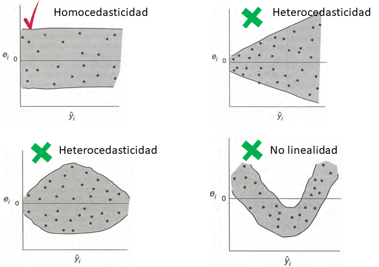
data_residuales <-
  data.frame(predichos = predichos_m1, residuales = residuales)


data_residuales |> 
  ggplot(aes(x = predichos, y = residuales)) +
  geom_point() +
  geom_hline(yintercept = 0, color = "red", linetype = 2) +
  geom_smooth(se = FALSE)

Validando otras predictoras

datos |> 
  pivot_longer(cols = -avg_price_milk) |> 
  ggplot(aes(x = value, y = avg_price_milk)) +
  facet_wrap(~name, ncol = 3, scales = "free_x") +
  geom_point() +
  geom_smooth(method = "lm")

Ajustando más modelos

modelo2 <- lm(avg_price_milk ~ alfalfa_hay_price, data = datos)
modelo3 <- lm(avg_price_milk ~ milk_feed_price_ratio, data = datos)
modelo4 <- lm(avg_price_milk ~ milk_per_cow, data = datos)

• ¿Cómo puedo comparar estos modelos?

AIC(modelo1, modelo2, modelo3, modelo4)

• Calculemos el RMSE de cada modelo:

predichos_m2 <- modelo2$fitted.values
predichos_m3 <- modelo3$fitted.values
predichos_m4 <- modelo4$fitted.values

rmse_vec(truth = valores_reales, estimate = predichos_m1)

[1] 0.01606818

rmse_vec(truth = valores_reales, estimate = predichos_m2)

[1] 0.01409574

rmse_vec(truth = valores_reales, estimate = predichos_m3)

[1] 0.02553965

rmse_vec(truth = valores_reales, estimate = predichos_m4)

[1] 0.0207514

Normalidad de residuales

Modelo 1

ggqqplot(modelo1$residuals)

Modelo 2

ggqqplot(modelo2$residuals)

Modelo 3

ggqqplot(modelo3$residuals)

Modelo 4

ggqqplot(modelo4$residuals)

Homocedasticidad

Modelo 1

data.frame(residuales = modelo1$residuals,
           predichos = modelo1$fitted.values) |>
  ggplot(aes(x = predichos, y = residuales)) +
  geom_point() +
  geom_hline(yintercept = 0,
             color = "red",
             linetype = 2) +
  geom_smooth(se = FALSE)

Modelo 2

data.frame(residuales = modelo2$residuals,
           predichos = modelo2$fitted.values) |>
  ggplot(aes(x = predichos, y = residuales)) +
  geom_point() +
  geom_hline(yintercept = 0,
             color = "red",
             linetype = 2) +
  geom_smooth(se = FALSE)

Modelo 3

data.frame(residuales = modelo3$residuals,
           predichos = modelo3$fitted.values) |>
  ggplot(aes(x = predichos, y = residuales)) +
  geom_point() +
  geom_hline(yintercept = 0,
             color = "red",
             linetype = 2) +
  geom_smooth(se = FALSE)

Modelo 4

data.frame(residuales = modelo4$residuals,
           predichos = modelo4$fitted.values) |>
  ggplot(aes(x = predichos, y = residuales)) +
  geom_point() +
  geom_hline(yintercept = 0,
             color = "red",
             linetype = 2) +
  geom_smooth(se = FALSE)